How To Make A Cashier Count Chart In Excel - Gggllpchr1h5sm. Stacked bar chart in excel. In my first example, i want to create a pie chart to see how many pens, rulers etc.i have sold in the month of april.simply follow the steps. As i mentioned, using excel table is the best way to create dynamic chart ranges. How to use the countif function in excel: You can select the data you want in the chart and press alt + f1 to create a chart immediately, but it might not be the best chart for the data.
When to use a line chart #1 use line charts when you want to show/focus on data trends (uptrend, downtrend, short term trend, sideways trend, long term) especially long term trends (i.e. You will see a list of chart types. Select insert > recommended charts. On the insert tab, in the charts group, click the line symbol. On the data tab, in the sort & filter group, click za.
Cdg Xiyhojsbsm from www.cours-gratuit.com Click the insert tab, click bar chart, and then click clustered bar (in 2016 versions, hover your cursor over the options to display a sample of how the chart will appear). Stacked bar chart in excel. The map chart in excel works best with large areas like counties, states, regions, countries, and continents. Changes over several months or years) between the values of the data series: How to create a stacked bar chart in excel? On the data tab, in the sort & filter group, click za. Use the tools in the picture group. Count values with conditions using this amazing function.
This is one of the most used and popular functions of excel that is used to lookup value from different ranges and sheets.
The organization chart templates add an org chart tab to the ribbon. The chart will appear on the same page as the data. All numbers including negative values, percentages, dates, fractions, and time are counted. Select the data range and click table under insert tab, see screenshot: These 50 shortcuts will make you work even faster on excel. How to use the vlookup function in excel: You can select the data you want in the chart and press alt + f1 to create a chart immediately, but it might not be the best chart for the data. Now you will show a select data source dialog box which will take input fields of data. The marks column will get sorted from smallest to largest. The map chart in excel works best with large areas like counties, states, regions, countries, and continents. This is one of the most used and popular functions of excel that is used to lookup value from different ranges and sheets. Using a graph is a great way to present your data in an effective, visual way. Select data for the chart.
First, select a number in column b. The simplest is to do a pivotchart. Count values with conditions using this amazing function. In this accelerated training, you'll learn how to use formulas to manipulate text, work with dates and times, lookup values with vlookup and index & match, count and sum with criteria, dynamically rank values, and create dynamic ranges. On the insert tab, in the charts group, click the line symbol.
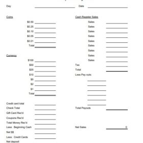
Yll I14mrzsfym from blog-assets.lightspeedhq.com Select the marks column and then go to home tab < sort & filter < sort smallest to largest. The free cashier balance sheet template for excel 2013 is a template for keeping track of a cashier's daily financial transactions, ensuring that all the money adds up by the end of the day. The select data source window will open. To create a line chart, execute the following steps. If the latter, only those cells that meet all of the specified conditions are counted. Select insert > recommended charts. This step is not required, but it will make the formulas easier to write. How to create a stacked bar chart in excel?
The free cashier balance sheet template for excel 2013 is a template for keeping track of a cashier's daily financial transactions, ensuring that all the money adds up by the end of the day.
The various chart options available to you will be listed under the charts section in the middle. And the data looks as below. The count function returns the count of numeric values in the list of supplied arguments. A simple chart in excel can say more than a sheet full of numbers. Select data and add series 5. I am using ms office 2010. Then click on add button and select e3:e6 in series values and keep series name blank. How to create a stacked bar chart in excel? Count values with conditions using this amazing function. You can use the countifs function in excel to count cells in a single range with a single condition as well as in multiple ranges with multiple conditions. Change layout, change shapes, and insert pictures. Select the marks column and then go to home tab < sort & filter < sort smallest to largest. Count values with conditions using this amazing function.
If the latter, only those cells that meet all of the specified conditions are counted. The various chart options available to you will be listed under the charts section in the middle. This tutorial will show you how to create stock charts in excel 2003. Excel stacked bar chart (table of contents) stacked bar chart in excel; A simple chart in excel can say more than a sheet full of numbers.
43hiz1pz4qmyrm from www.excelstemplates.com Formulas are the key to getting things done in excel. As you can see in the screenshot below, start date is already added under legend entries (series).and you need to add duration there as well. 2) next, from the top menu in your excel workbook, select the insert tab. Select the data range and click table under insert tab, see screenshot: You can select the data you want in the chart and press alt + f1 to create a chart immediately, but it might not be the best chart for the data. How to use the countif function in excel: It easily and clearly shows if the register or drawer comes short or over. This helps you to represent data in a stacked manner.
If the specific day of the month is inconsequential, such as the billing date for monthly bills.
If the latter, only those cells that meet all of the specified conditions are counted. Using a graph is a great way to present your data in an effective, visual way. Add duration data to the chart. Stacked bar chart in excel. 1) first, select the data for the chart, like this. First, select a number in column b. However, if you can't use excel table for some reason (possibly if you are using excel 2003), there is another (slightly complicated) way to create dynamic chart ranges using excel formulas and named ranges. The layout and arrange groups have tools for changing the layout and hierarchy of the shapes. On a mac, you'll instead click the design tab, click add chart element, select chart title, click a location, and type in the graph's title. In this video tutorial, you'll see how to create a simple pie graph in excel. How to make a cashier count chart in excel. Click the insert tab, click bar chart, and then click clustered bar (in 2016 versions, hover your cursor over the options to display a sample of how the chart will appear). Use the tools in the picture group.